캐글코리아 Spooky NLP and Topic Modelling tutorial

라이브러리 임포트

import base64
import numpy as np
import pandas as pd

# Plotly imports
import plotly.offline as py
py.init_notebook_mode(connected=True)
import plotly.graph_objs as go
import plotly.tools as tls

# Other imports
from collections import Counter
from scipy.misc import imread

from sklearn.feature_extraction.text import TfidfVectorizer, CountVectorizer
from sklearn.decomposition import NMF, LatentDirichletAllocation
from matplotlib import pyplot as plt
%matplotlib inline

 

데이터 받기

# Loading in the training data with Pandas
train = pd.read_csv("/kaggle/input/spooky/train.csv")
train.head()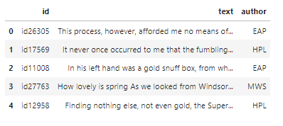

train['author'].unique()

저자별 통계 시각화 하기

import plotly.graph_objs as go
z = {'EAP': 'Edgar Allen Poe', 'MWS': 'Mary Shelley', 'HPL': 'HP Lovecraft'}
data = [go.Bar(
            x = train.author.map(z).unique(),
            y = train.author.value_counts().values,
            marker= dict(colorscale='Jet',
                         color = train.author.value_counts().values
                        ),
            text='Text entries attributed to Author'
    )]

layout = go.Layout(
    title='Target variable distribution'
)

fig = go.Figure(data=data, layout=layout)

py.iplot(fig, filename='basic-bar')

단어의 갯수를 새어서 반환하여 시각화 합니다.

all_words = train['text'].str.split(expand=True).unstack().value_counts()
data = [go.Bar(
            x = all_words.index.values[2:50],
            y = all_words.values[2:50],
            marker= dict(colorscale='Jet',
                         color = all_words.values[2:100]
                        ),
            text='Word counts'
    )]

layout = go.Layout(
    title='Top 50 (Uncleaned) Word frequencies in the training dataset'
)

fig = go.Figure(data=data, layout=layout)

py.iplot(fig, filename='basic-bar')

해당작가의 텍스트를 변수에 array형식으로 넣습니다.

eap = train[train.author=="EAP"]["text"].values
hpl = train[train.author=="HPL"]["text"].values
mws = train[train.author=="MWS"]["text"].values

단어를 공백을 기준으로 나누기

train.text.values[0]은 첫번쨰 인덱스의 text컬럼을 가져온다

# Storing the first text element as a string
first_text = train.text.values[0]
print(first_text)
print("="*90)
print(first_text.split(" "))

토크나이저를 통해서 단어 분리하기

first_text_list = nltk.word_tokenize(first_text)
print(first_text_list)

내장된 불용어 갯수 출력하기

stopwords = nltk.corpus.stopwords.words('english')
len(stopwords)

불용어 제거 코드

원리는 단어마다 lower이라는 함수를 적용한뒤 불용어와 다른 텍스트라면 남겨두는 방식이다.

first_text_list_cleaned = [word for word in first_text_list if word.lower() not in stopwords]
print(first_text_list_cleaned)
print("="*90)
print("Length of original list: {0} words\n"
      "Length of list after stopwords removal: {1} words"
      .format(len(first_text_list), len(first_text_list_cleaned)))

포터 알고리즘 사용하기

포터알고리즘을 통해서 어간만 추출하였음

stemmer = nltk.stem.PorterStemmer()
print("The stemmed form of running is: {}".format(stemmer.stem("running")))
print("The stemmed form of runs is: {}".format(stemmer.stem("runs")))
print("The stemmed form of run is: {}".format(stemmer.stem("run")))

가장 가까운 표제어로 바꾸기

워드넷 레마타이저사용하기

from nltk.stem import WordNetLemmatizer
lemm = WordNetLemmatizer()
print("The lemmatized form of leaves is: {}".format(lemm.lemmatize("leaves")))

tf-idf 적용 

# Defining our sentence
sentence = ["I love to eat Burgers", 
            "I love to eat Fries"]
vectorizer = CountVectorizer(min_df=0)
sentence_transform = vectorizer.fit_transform(sentence)

 

id-idf 출력

get_feature_names()는 단어 리스트를 가져옴

toarray()는 tf-idf결과를 가져옴

print("The features are:\n {}".format(vectorizer.get_feature_names()))
print("\nThe vectorized array looks like:\n {}".format(sentence_transform.toarray()))

상위 단어를 지정하여 가져옴

# Define helper function to print top words
def print_top_words(model, feature_names, n_top_words):
    for index, topic in enumerate(model.components_):
        message = "\nTopic #{}:".format(index)
        message += " ".join([feature_names[i] for i in topic.argsort()[:-n_top_words - 1 :-1]])
        print(message)
        print("="*70)

 

표제어로 변환후 tf-idf를 적용함

lemm = WordNetLemmatizer()
class LemmaCountVectorizer(CountVectorizer):
    def build_analyzer(self):
        analyzer = super(LemmaCountVectorizer, self).build_analyzer()
        return lambda doc: (lemm.lemmatize(w) for w in analyzer(doc))

 

표제어 tf-idf함수 적용

# Storing the entire training text in a list
text = list(train.text.values)
# Calling our overwritten Count vectorizer
tf_vectorizer = LemmaCountVectorizer(max_df=0.95, 
                                     min_df=2,
                                     stop_words='english',
                                     decode_error='ignore')
tf = tf_vectorizer.fit_transform(text)

단어 별 중요도 시각화

feature_names = tf_vectorizer.get_feature_names()
count_vec = np.asarray(tf.sum(axis=0)).ravel()
zipped = list(zip(feature_names, count_vec))
x, y = (list(x) for x in zip(*sorted(zipped, key=lambda x: x[1], reverse=True)))
# Now I want to extract out on the top 15 and bottom 15 words
Y = np.concatenate([y[0:15], y[-16:-1]])
X = np.concatenate([x[0:15], x[-16:-1]])

# Plotting the Plot.ly plot for the Top 50 word frequencies
data = [go.Bar(
            x = x[0:50],
            y = y[0:50],
            marker= dict(colorscale='Jet',
                         color = y[0:50]
                        ),
            text='Word counts'
    )]

layout = go.Layout(
    title='Top 50 Word frequencies after Preprocessing'
)

fig = go.Figure(data=data, layout=layout)

py.iplot(fig, filename='basic-bar')

# Plotting the Plot.ly plot for the Top 50 word frequencies
data = [go.Bar(
            x = x[-100:],
            y = y[-100:],
            marker= dict(colorscale='Portland',
                         color = y[-100:]
                        ),
            text='Word counts'
    )]

layout = go.Layout(
    title='Bottom 100 Word frequencies after Preprocessing'
)

fig = go.Figure(data=data, layout=layout)

py.iplot(fig, filename='basic-bar')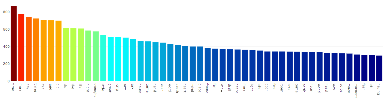

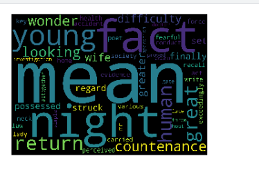
워드 클라우드를 통한 시각화

first_topic_words변수의 단어를 시각화해줌

# Generating the wordcloud with the values under the category dataframe
firstcloud = WordCloud(
                          stopwords=STOPWORDS,
                          background_color='black',
                          width=2500,
                          height=1800
                         ).generate(" ".join(first_topic_words))
plt.imshow(firstcloud)
plt.axis('off')
plt.show()