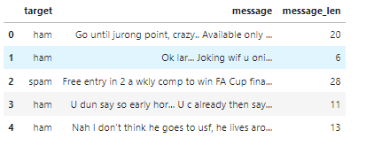
데이터 받기
df = pd.read_csv("/kaggle/input/sms-spam-collection-dataset/spam.csv", encoding="latin-1")
df = df.dropna(how="any", axis=1)
df.columns = ['target', 'message']
df.head()

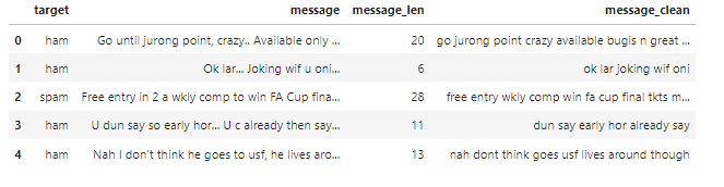
메시지 길어 컬럼 만들기
df['message_len'] = df['message'].apply(lambda x: len(x.split(' ')))
df.head()
agg를 통한 통계 기법
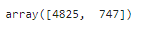
balance_counts = df.groupby('target')['target'].agg('count').values
balance_counts
스팸빈도 시각화
fig = go.Figure()
fig.add_trace(go.Bar(
x=['ham'],
y=[balance_counts[0]],
name='ham',
text=[balance_counts[0]],
textposition='auto',
marker_color=primary_blue
))
fig.add_trace(go.Bar(
x=['spam'],
y=[balance_counts[1]],
name='spam',
text=[balance_counts[1]],
textposition='auto',
marker_color=primary_grey
))
fig.update_layout(
title='<span style="font-size:32px; font-family:Times New Roman">Dataset distribution by target</span>'
)
fig.show()
문자길이에따른 스팸여부 시각화
ham_df = df[df['target'] == 'ham']['message_len'].value_counts().sort_index()
spam_df = df[df['target'] == 'spam']['message_len'].value_counts().sort_index()
fig = go.Figure()
fig.add_trace(go.Scatter(
x=ham_df.index,
y=ham_df.values,
name='ham',
fill='tozeroy',
marker_color=primary_blue,
))
fig.add_trace(go.Scatter(
x=spam_df.index,
y=spam_df.values,
name='spam',
fill='tozeroy',
marker_color=primary_grey,
))
fig.update_layout(
title='<span style="font-size:32px; font-family:Times New Roman">Data Roles in Different Fields</span>'
)
fig.update_xaxes(range=[0, 70])
fig.show()

정규표현식을 통한 특수문자 제거 구현
def clean_text(text):
'''Make text lowercase, remove text in square brackets,remove links,remove punctuation
and remove words containing numbers.'''
text = str(text).lower()
text = re.sub('\[.*?\]', '', text)
text = re.sub('https?://\S+|www\.\S+', '', text)
text = re.sub('<.*?>+', '', text)
text = re.sub('[%s]' % re.escape(string.punctuation), '', text)
text = re.sub('\n', '', text)
text = re.sub('\w*\d\w*', '', text)
return text
df['message_clean'] = df['message'].apply(clean_text)
df.head()

불용어 제거
stop_words = stopwords.words('english')
more_stopwords = ['u', 'im', 'c']
stop_words = stop_words + more_stopwords
def remove_stopwords(text):
text = ' '.join(word for word in text.split(' ') if word not in stop_words)
return text
df['message_clean'] = df['message_clean'].apply(remove_stopwords)
df.head()
형태소 분석
stemmer = nltk.SnowballStemmer("english")
def stemm_text(text):
text = ' '.join(stemmer.stem(word) for word in text.split(' '))
return text
df['message_clean'] = df['message_clean'].apply(stemm_text)
df.head()

위과정 요약 코드
def preprocess_data(text):
# Clean puntuation, urls, and so on
text = clean_text(text)
# Remove stopwords
text = ' '.join(word for word in text.split(' ') if word not in stop_words)
# Stemm all the words in the sentence
text = ' '.join(stemmer.stem(word) for word in text.split(' '))
return text
df['message_clean'] = df['message_clean'].apply(preprocess_data)
df.head()
타겟을 0또는 1이라는 숫자로 바꾸기
from sklearn.preprocessing import LabelEncoder
le = LabelEncoder()
le.fit(df['target'])
df['target_encoded'] = le.transform(df['target'])
df.head()

ham인 경우 시각화
twitter_mask = np.array(Image.open('/kaggle/input/masksforwordclouds/twitter_mask3.jpg'))
wc = WordCloud(
background_color='white',
max_words=200,
mask=twitter_mask,
)
wc.generate(' '.join(text for text in df.loc[df['target'] == 'ham', 'message_clean']))
plt.figure(figsize=(18,10))
plt.title('Top words for HAM messages',
fontdict={'size': 22, 'verticalalignment': 'bottom'})
plt.imshow(wc)
plt.axis("off")
plt.show()

spam인 경우 시각화
twitter_mask = np.array(Image.open('/kaggle/input/masksforwordclouds/twitter_mask3.jpg'))
wc = WordCloud(
background_color='white',
max_words=200,
mask=twitter_mask,
)
wc.generate(' '.join(text for text in df.loc[df['target'] == 'spam', 'message_clean']))
plt.figure(figsize=(18,10))
plt.title('Top words for SPAM messages',
fontdict={'size': 22, 'verticalalignment': 'bottom'})
plt.imshow(wc)
plt.axis("off")
plt.show()

테스트 데이터와 학습데이터로 나누기
x = df['message_clean']
y = df['target_encoded']
print(len(x), len(y))
from sklearn.model_selection import train_test_split
x_train, x_test, y_train, y_test = train_test_split(x, y, random_state=42)
print(len(x_train), len(y_train))
print(len(x_test), len(y_test))
tf-idfcounter 적용
from sklearn.feature_extraction.text import CountVectorizer
vect = CountVectorizer()
vect.fit(x_train)
x_train_dtm = vect.transform(x_train)
x_test_dtm = vect.transform(x_test)
tf-idf counter 선언
# 추출할 최대 상위 100개로 제한함
#어휘에 포함될 최소 용어는 제한 최대 70%까지 용어 제한하겠음
# 최소 10%까지만 제한 하겠다는 의미
즉 10~70%사이만 제외하겠다는 의미임
# ngram_range=(1,2)은 단어묶음을 하나또는 두개로 하라는 의미임
vect_tunned = CountVectorizer(stop_words='english', ngram_range=(1,2), min_df=0.1, max_df=0.7, max_features=100)
vect_tunned
예시 그림

tf-idf vector적용하기
from sklearn.feature_extraction.text import TfidfTransformer
tfidf_transformer = TfidfTransformer()
tfidf_transformer.fit(x_train_dtm)
x_train_tfidf = tfidf_transformer.transform(x_train_dtm)
x_train_tfidf
texts = df['message_clean']
target = df['target_encoded']
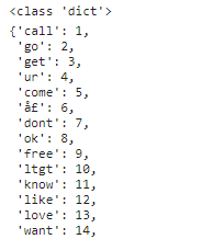
토크나이저 적용하기
word_tokenizer = Tokenizer()
#텍스트 추가하기
#dict형태로 이루어질예정임
word_tokenizer.fit_on_texts(texts)
#처음인덱스는 0으로 시작하기에 +1추가하기
#word_index는 dict사전임
vocab_length = len(word_tokenizer.word_index) + 1
vocab_length
print(type(word_tokenizer.word_index))
word_tokenizer.word_index
임베딩하기
def embed(corpus):
return word_tokenizer.texts_to_sequences(corpus)
longest_train = max(texts, key=lambda sentence: len(word_tokenize(sentence)))
length_long_sentence = len(word_tokenize(longest_train))
train_padded_sentences = pad_sequences(
embed(texts),
length_long_sentence,
padding='post'
)
train_padded_sentences

dict안에 값을 비교하여 원하는 값이 있다면 출력하기
embeddings_dictionary = dict()
embedding_dim = 100
with open('/kaggle/input/glove6b100dtxt/glove.6B.100d.txt') as fp:
for line in fp.readlines():
records = line.split()
word = records[0]
vector_dimensions = np.asarray(records[1:], dtype='float32')
embeddings_dictionary [word] = vector_dimensions
embedding_matrix = np.zeros((vocab_length, embedding_dim))
for word, index in word_tokenizer.word_index.items():
embedding_vector = embeddings_dictionary.get(word)
if embedding_vector is not None:
embedding_matrix[index] = embedding_vector
embedding_matrix
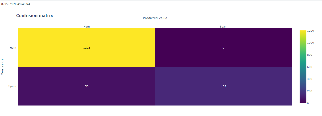
혼돈행렬 시각화 구현코드
import plotly.figure_factory as ff
x_axes = ['Ham', 'Spam']
y_axes = ['Spam', 'Ham']
def conf_matrix(z, x=x_axes, y=y_axes):
#값 거꾸로 뒤집기
#0이기에 수직임
z = np.flip(z, 0)
z_text = [[str(y) for y in x] for x in z]
# 시각화
# x열
# y행
# annotation_text는 텍스트
# colorscale는 색깔
fig = ff.create_annotated_heatmap(z, x=x, y=y, annotation_text=z_text, colorscale='Viridis')
# add title
fig.update_layout(title_text='<b>Confusion matrix</b>',
xaxis = dict(title='Predicted value'),
yaxis = dict(title='Real value')
)
# add colorbar
fig['data'][0]['showscale'] = True
return fig
나이즈 베이 모델로 학습진행
from sklearn.naive_bayes import MultinomialNB
nb = MultinomialNB()
# Train the model
nb.fit(x_train_dtm, y_train)
예측 출력
y_pred_class = nb.predict(x_test_dtm)
y_pred_prob = nb.predict_proba(x_test_dtm)[:, 1]
예측 혼돈행렬로 출력
from sklearn import metrics
print(metrics.accuracy_score(y_test, y_pred_class))
conf_matrix(metrics.confusion_matrix(y_test, y_pred_class))
정확도 출력
metrics.roc_auc_score(y_test, y_pred_prob)
나이브 베이 파이프라인 정확도 출력
from sklearn.feature_extraction.text import TfidfTransformer
from sklearn.pipeline import Pipeline
pipe = Pipeline([('bow', CountVectorizer()),
('tfid', TfidfTransformer()),
('model', MultinomialNB())])
pipe.fit(x_train, y_train)
y_pred_class = pipe.predict(x_test)
print(metrics.accuracy_score(y_test, y_pred_class))
conf_matrix(metrics.confusion_matrix(y_test, y_pred_class))
X-bost 파이프라인 정확도 출력
import xgboost as xgb
pipe = Pipeline([
('bow', CountVectorizer()),
('tfid', TfidfTransformer()),
('model', xgb.XGBClassifier(
learning_rate=0.1,
max_depth=7,
n_estimators=80,
use_label_encoder=False,
eval_metric='auc',
# colsample_bytree=0.8,
# subsample=0.7,
# min_child_weight=5,
))
])
pipe.fit(x_train, y_train)
y_pred_class = pipe.predict(x_test)
y_pred_train = pipe.predict(x_train)
print('Train: {}'.format(metrics.accuracy_score(y_train, y_pred_train)))
print('Test: {}'.format(metrics.accuracy_score(y_test, y_pred_class)))
conf_matrix(metrics.confusion_matrix(y_test, y_pred_class))

lsmt 모델 요약
X_train, X_test, y_train, y_test = train_test_split(
train_padded_sentences,
target,
test_size=0.25
)
def glove_lstm():
model = Sequential()
model.add(Embedding(
input_dim=embedding_matrix.shape[0],
output_dim=embedding_matrix.shape[1],
weights = [embedding_matrix],
input_length=length_long_sentence
))
model.add(Bidirectional(LSTM(
length_long_sentence,
return_sequences = True,
recurrent_dropout=0.2
)))
model.add(GlobalMaxPool1D())
model.add(BatchNormalization())
model.add(Dropout(0.5))
model.add(Dense(length_long_sentence, activation = "relu"))
model.add(Dropout(0.5))
model.add(Dense(length_long_sentence, activation = "relu"))
model.add(Dropout(0.5))
model.add(Dense(1, activation = 'sigmoid'))
model.compile(optimizer='rmsprop', loss='binary_crossentropy', metrics=['accuracy'])
return model
model = glove_lstm()
model.summary()

lsmt 모델 학습
model = glove_lstm()
checkpoint = ModelCheckpoint(
'model.h5',
monitor = 'val_loss',
verbose = 1,
save_best_only = True
)
reduce_lr = ReduceLROnPlateau(
monitor = 'val_loss',
factor = 0.2,
verbose = 1,
patience = 5,
min_lr = 0.001
)
history = model.fit(
X_train,
y_train,
epochs = 7,
batch_size = 32,
validation_data = (X_test, y_test),
verbose = 1,
callbacks = [reduce_lr, checkpoint]
)

시각화 함수 구현
def plot_learning_curves(history, arr):
fig, ax = plt.subplots(1, 2, figsize=(20, 5))
for idx in range(2):
ax[idx].plot(history.history[arr[idx][0]])
ax[idx].plot(history.history[arr[idx][1]])
ax[idx].legend([arr[idx][0], arr[idx][1]],fontsize=18)
ax[idx].set_xlabel('A ',fontsize=16)
ax[idx].set_ylabel('B',fontsize=16)
ax[idx].set_title(arr[idx][0] + ' X ' + arr[idx][1],fontsize=16)
plot_learning_curves(history, [['loss', 'val_loss'],['accuracy', 'val_accuracy']])

혼돈 행렬 출력
y_preds = (model.predict(X_test) > 0.5).astype("int32")
conf_matrix(metrics.confusion_matrix(y_test, y_preds))
bert 사용하기
!pip install transformers
import tensorflow as tf
from tensorflow.keras.layers import Dense, Input
from tensorflow.keras.optimizers import Adam
from tensorflow.keras.models import Model
from tensorflow.keras.callbacks import ModelCheckpoint
import transformers
from tqdm.notebook import tqdm
from tokenizers import BertWordPieceTokenizer
try:
tpu = tf.distribute.cluster_resolver.TPUClusterResolver()
tf.config.experimental_connect_to_cluster(tpu)
tf.tpu.experimental.initialize_tpu_system(tpu)
strategy = tf.distribute.experimental.TPUStrategy(tpu)
except:
strategy = tf.distribute.get_strategy()
print('Number of replicas in sync: ', strategy.num_replicas_in_sync)
from transformers import BertTokenizer
tokenizer = BertTokenizer.from_pretrained('bert-large-uncased')
def bert_encode(data, maximum_length) :
input_ids = []
attention_masks = []
for text in data:
encoded = tokenizer.encode_plus(
text,
add_special_tokens=True,
max_length=maximum_length,
pad_to_max_length=True,
return_attention_mask=True,
)
input_ids.append(encoded['input_ids'])
attention_masks.append(encoded['attention_mask'])
return np.array(input_ids),np.array(attention_masks)
texts = df['message_clean']
target = df['target_encoded']
train_input_ids, train_attention_masks = bert_encode(texts,60)
import tensorflow as tf
from tensorflow.keras.optimizers import Adam
def create_model(bert_model):
input_ids = tf.keras.Input(shape=(60,),dtype='int32')
attention_masks = tf.keras.Input(shape=(60,),dtype='int32')
output = bert_model([input_ids,attention_masks])
output = output[1]
output = tf.keras.layers.Dense(32,activation='relu')(output)
output = tf.keras.layers.Dropout(0.2)(output)
output = tf.keras.layers.Dense(1,activation='sigmoid')(output)
model = tf.keras.models.Model(inputs = [input_ids,attention_masks],outputs = output)
model.compile(Adam(lr=1e-5), loss='binary_crossentropy', metrics=['accuracy'])
return model
from transformers import TFBertModel
bert_model = TFBertModel.from_pretrained('bert-base-uncased')
model = create_model(bert_model)
model.summary()

history = model.fit(
[train_input_ids, train_attention_masks],
target,
validation_split=0.2,
epochs=3,
batch_size=10
)
plot_learning_curves(history, [['loss', 'val_loss'],['accuracy', 'val_accuracy']])

'캐글 코드' 카테고리의 다른 글
| 캐글 우주 타이타닉 예측 1탄 (0) | 2024.02.23 |
|---|---|
| 캐글 자전거 수요예측 (0) | 2024.02.22 |
| 캐글 SMS Spam Collection Dataset 1탄 (0) | 2024.01.31 |
| 캐글 News Detection 1탄 (1) | 2024.01.30 |
| 캐글 NLP 뉴스데이터 분석 1탄 (0) | 2024.01.29 |


